RINalyzer Tutorials
Tutorials for Cytoscape 3.x
Tutorials for Cytoscape 2.x
Download the video tutorial here or watch it online now. Detailed instructions are given below.
In the following, screenshots for each step appear when hovering the mouse over (image). If you cannot see the whole image, you can use the keyboard arrows to move to the right or to the bottom while holding the mouse over the image.
Prepare data
For this tutorial, we will use the protein structure of the human deoxyhaemoglobin with PDB identifier 4hhb. We will compare one of the α subunits with one of the β subunits, i.e., chain A with chain B, but we will refer to them as two different structures.
- Get a structure alignment file using the RCSB PDB Protein Comparison Tool.
- Go to the RCSB PDB Protein Comparison Tool web site (image
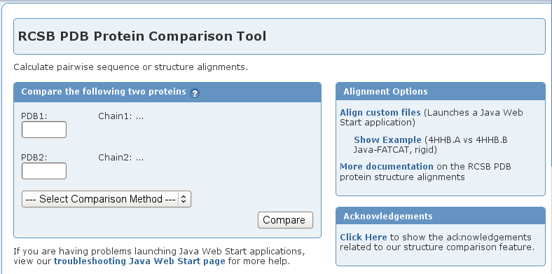 ).
).
- Enter 4hhb in the text field for PDB1 and the tool will automatically select chain A (image
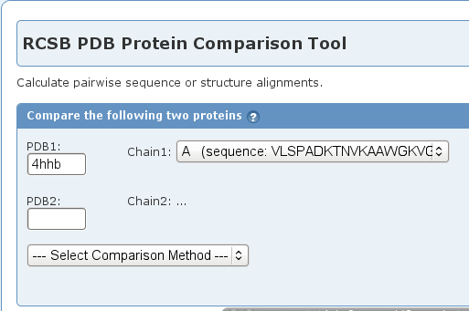 ).
).
- Enter the same identifier in the text field for PDB2 and select chain B from the drop-down menu (image
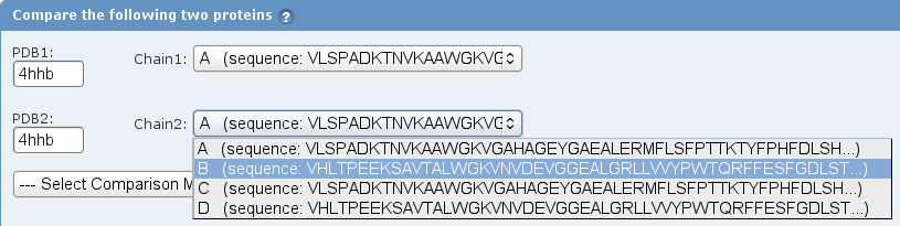 ).
).
- In the Select Comparison Method drop-down menu, choose the jCE algorithm (image
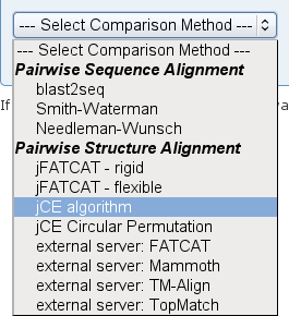 ).
).
- Click the Compare button (image
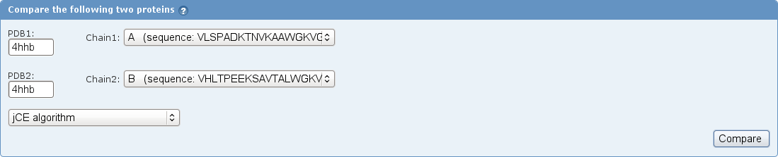 ).
).
- If you want you may allow your browser to run the Java application for visualizing the structure alignment with Jmol by clicking the Run button (image
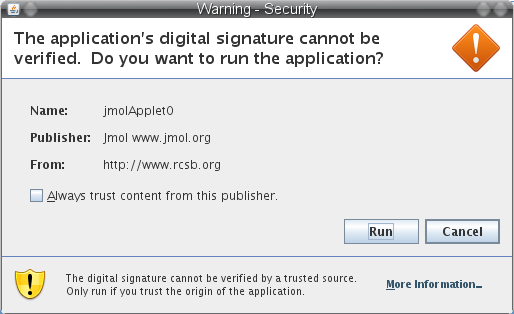 ).
).
- Scroll down to the Download Alignment panel (image
 ). Right-click the link Download XML and select the option Save Link As... (image
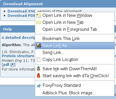 ).
).
- In the file browser, select a directory where the file should be saved, enter a name for it, e.g., 4hhbA_vs_4hhbB.xml, and click the Save button (image
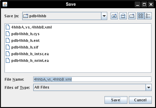 ).
).
- Close the Protein Comparison Tool.
- Download the RIN data for PDB entry 4hhb and open the corresponding RIN in Cytoscape following the instructions in Tutorial 1 until the layout is applied on the network view.
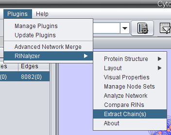
- Extract chain A and chain B as new networks.
- In Cytoscape, go to Plugins → RINalyzer → Extract chain(s) (image
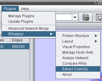 ).
).
- Check the box of chain A, enter a name for the new network, e.g., pdb4hhb_A, and click the OK button (image
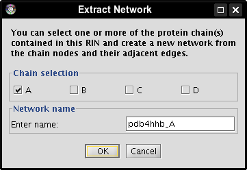 ). A new network is created that contains all nodes belonging to chain A (image
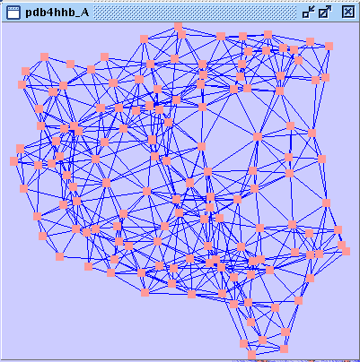 ).
).
- In the Control Panel, select network pdb4hhb_h.sif (image
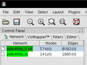 ).
).
- Go to Plugins → RINalyzer → Extract chain(s) (image
 ).
).
- Check the box of chain B, enter a name for the new network, e.g., pdb4hhb_B, and click the OK button (image
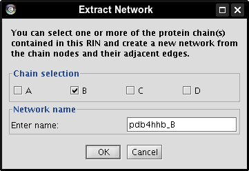 ). A new network is created that contains all nodes belonging to chain B (image
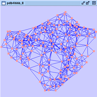 ).
).
- You can apply a layout to both networks and customize their visual properties (go to Plugins → RINalyzer → Visual Properties). The Organic layout by yFiles (go to Layout → yFiles → Organic) can be useful in case you do not want to open the corresponding 3D structure in Chimera, which is a precondition for applying the RINLayout.
Perform comparison
- Go to Plugins → RINalyzer → Compare RINs (image
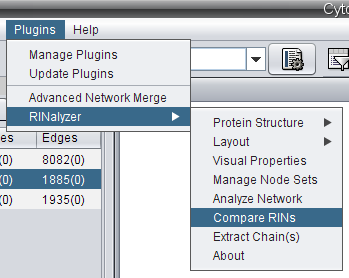 ).
).
- Select network pdb4hhb_A as first network (image
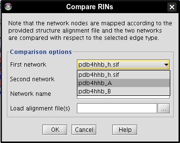 ), network pdb4hhb_B as second network (image
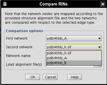 ), enter a name for the new network, e.g., comparison (image
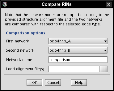 ).
).
- Click the ... button (image
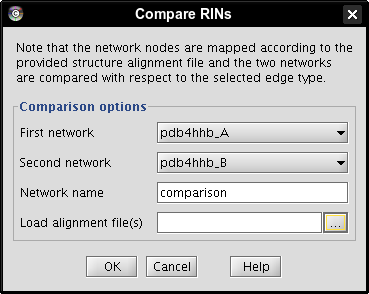 ) and open the alignment file downloaded earlier (image
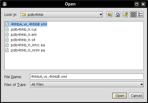 ).
).
- Click the Compare button to perform the comparison (image
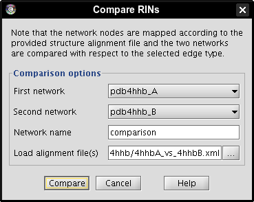 ).
).
- A new network with 148 nodes and 2405 edges is created. You can maximize the network view window (image
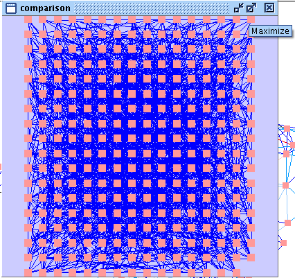 ), apply the organic layout and the RIN visual properties.
- If you use Cytoscape 2.6.x, the network should look as in this image
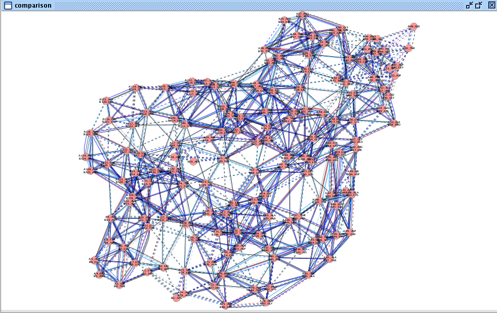 . The solid edge lines represent residue interactions present in both networks, while the dashed edge lines are interactions found in only one of the structures. If you use Cytoscape 2.7 and above, then you will observe three different edge line styles as in this image
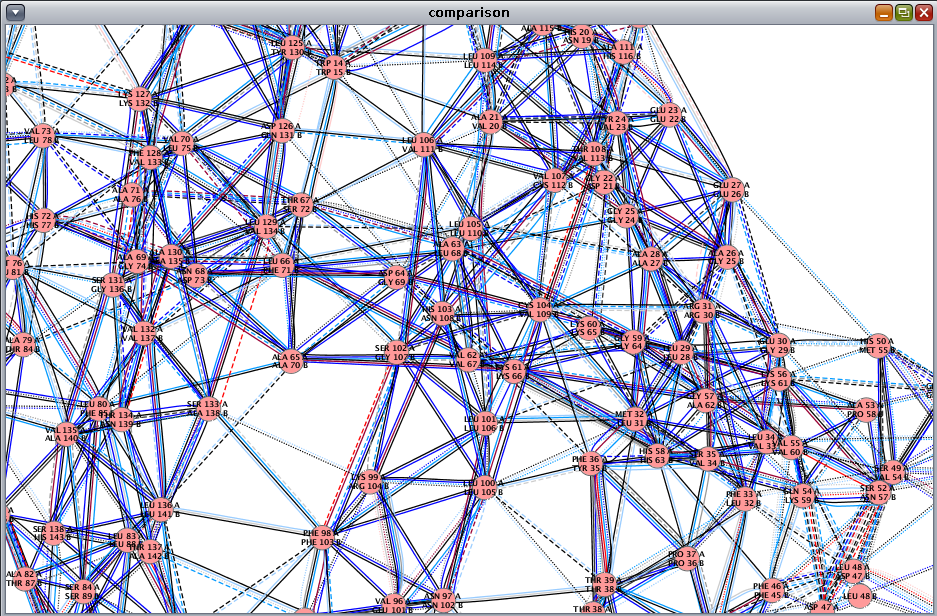 : solid lines for interactions present in both networks, dashed lines for network 1, and dotted lines for network 2.
- Customize the network view for interpreting the result:
- Go to Plugins → RINalyzer → Visual Properties and select the Edges tab (image
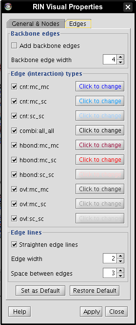 ).
).
- Hide all edges except combi:all_all by unchecking the boxes beside each edge type and close the RIN Visual Properties dialog (image
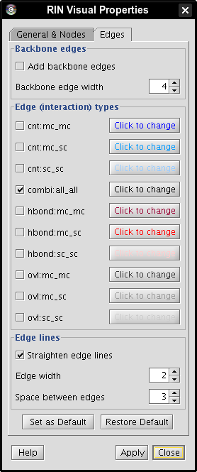 ).
).
- In the Control Panel, go to VizMapper (image
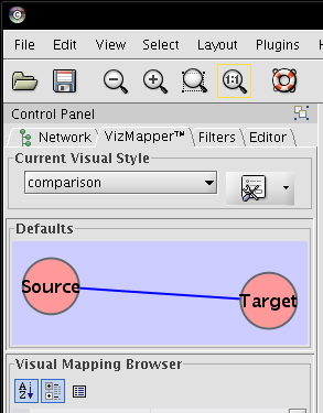 ).
).
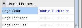
- Double-click the field Edge Color (image
 ), select the attribute BelongsTo (image
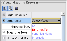 ) and the mapping type Discrete Mapping (image
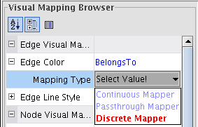 ).
).
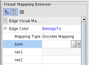
- For each attribute: click on the field beside the attribute and then on the appeared ... button (image
 ); select a color and click OK (image
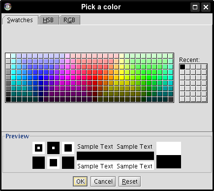 ). We picked black for edges in both networks, green for edges in the first network, and red for edges in the second (image
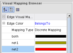 ).
).
- Repeat the same actions for mapping the node color using the BelongsTo attribute (image
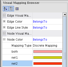 ).
).
- Click on the field beside the visual property Node Label and select the attribute CombinedLabel (image
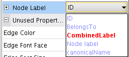 ).
).
- Now, all node labels are composed of the node labels of the nodes from the compared networks (image
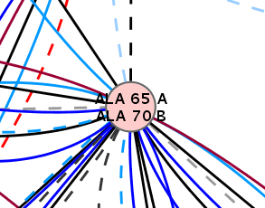 ).
).
- Now, the network looks as in this image
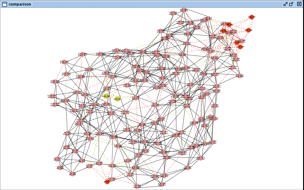 (in Cytoscape 2.6.x) and by zooming-in you can observe the residue interaction differences between the superimposed α and β subunits of the human deoxyhaemoglobin.